Description

This article introduces both a new algorithm for reconstructing epsilon-machines from data, as well as the decisional states. These are defined as the internal states of a system that lead to the same decision, based on a user-provided utility or pay-off function. The utility function encodes some a priori knowledge external to the system, it quantifies how bad it is to make mistakes. The intrinsic underlying structure of the system is modeled by an epsilon-machine and its causal states. The decisional states form a partition of the lower-level causal states that is defined according to the higher-level user's knowledge. In a complex systems perspective, the decisional states are thus the "emerging" patterns corresponding to the utility function. The transitions between these decisional states correspond to events that lead to a change of decision. The new REMAPF algorithm estimates both the epsilon-machine and the decisional states from data. Application examples are given for hidden model reconstruction, cellular automata filtering, and edge detection in images.

The main contributions of this article are:

A practical algorithm for computing the system states from data, which as an intermediate step reconstructs the epsilon-machine.
The way information is encoded in the utility function, which represents a new and clear way to represent the user knowledge independently of the system's intrinsic dynamics.
The decisional states concept, allowing a modeller to represent system states with equivalent decisions for the user based on the preceeding utility function.

Source code of the reference implementation is available as Free/Libre software.

You may also be interested by a related previous work where data can be incrementally added and removed in order to maintain the current estimates of the causal states of the system. See the dedicated page on this site.

Short explanation

Predictions in a physical context

In a physical framework information transfer is limited by the speed of light. In this view the system present is a single point in state-space. Contrast this with dynamical systems where the present is the whole state vector, the line in the figure below. Here there is no instant propagation of information, and only a small portion of the state vector is accessible.

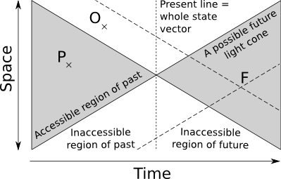
The past light-cone is the collection of all points that could possibly have an a priori causal influence on the present. The future cone is the collection of all points that might possibly be influenced by the present state. The problem is that in order to infer correctly the state of a point F in the future cone we might potentially need all points in the past light cone of F. It would theoretically be possible to have access to the points like P in the system current past, provided in practice that we indeed recorded the value of P. However there is by definition no way of getting the value of points like O that are outside the current system past light cone. Since both points belong to the past light cone of a point F in our own future, the consequence is that even for deterministic systems we get a statistical distribution of possible futures for a given observed past, depending on what information present outside the current past cone is necessary to predict the future. In other words, boundary and/or conditions in inaccessible regions may determine part of the future.

Let us now consider grouping two past cones x₁^- and x₂^- together if they lead to the same distribution of futures p(x⁺|x₁^-)=p(x⁺|x₂^-). Suppose that point P in the past have a distinct value for pasts x₁^- and x₂^-. Then there is no way to recover what the value of P was by new observations: we cannot use future knowledge to decide between x₁^- and x₂^- since p(x⁺|x₁^-)=p(x⁺|x₂^-). For all practical matter these two pasts are then equivalent. Mathematically the associated equivalence relation x₁^- ≡ x₂^- partitions the system past light cones in sets σ(x^-)={ y^-: p(x⁺|y^-)=p(x⁺|x^-)}.

The sets σ are called the causal states of the system (see Cosma Shalizi's Thesis). In a discrete setup a new observation leads to a transition from a state σ₁ to a state σ₂. The causal states and their transitions form a deterministic automaton: the ε-machine (see this article by James Crutchfield and Karl Young). A neat result is the abstraction of the time dependencies into the states. The transitions between states include all dependencies from the past that could have an influence on the future, hence the ε-machine actually forms a Markovian graph.

The causal states construction is not limited to light-cones as described above. We can also cluster together data (parameter) points x∊X according to the conditional distributions p(Z|x) of points z∊Z in a space of predictions. The same equivalence relation as above can be defined: The equivalence classes induced by this relation might also be called causal states by analogy, even though no causality relation needs to be explicitly introduced as is the case for light-cones.

Introduction of the utility function

The preceeding view offers no distinction between futures with dire or benign consequences. For example, administrating a drug to a patient may cause severe secondary effects. The causal states view is to monitor p(effect|drug), but does not specify if the effect is desired or not. In practice this simple example would need to take into account much more parameters, like the patient condition when administrating the drug, etc. But this is an illustration only, where we wish to predict an effect (space Z) from a drug (space X).

The idea is to introduce a utility function U(y,z) that tells the consequence of predicting y∊Z (the patient state we think will happen) instead of z (the patient state that really happens). For example, if we administrate the drug because we think this will solve the patient headache, but she gets an additionnal bellyache instead, then the utility of that prediction is not very good.

What happens when we now put together drugs X according to their expected utility E[U(effect|drug)]=E[U(y|x)]=∫_z∊ZU(y,z)p(z|x) instead of the probabilities p(effect|drug) ? We actually need to distinguish two cases:

We put x₁ and x₂ together when the expected effect that achieve the maximal utility is the same. This allows to classify drugs by category, like treating headaches or treating bellyaches. But tells nothing about secondary effects.
We put together drugs x₁ and x₂ when the expected utility is the same, irrespectively of what the drug is for. This allows to classify drugs according to their effectiveness, and keep the most powerful drugs out of self-medication. This tells nothing about what the drug is for in the first place.
We put together drugs according to both above criteria at the same time.

Technically speaking:

The first case is x₁ ≡ x₂ when argmax_y∊ZE[U(y|x₁)]=argmax_y∊ZE[U(y|x₁)]. This is the iso-prediction state.
The second case is x₁ ≡ x₂ when max_y∊ZE[U(y|x₁)]=max_y∊ZE[U(y|x₁)]. This is the iso-utility state.
The third state is the intersection of both. This is the decisional state.

The article gives more details. The name "decisional state" comes from the assumption the utility function encodes all the user needs to know in order to make a decision. The transitions between the decisional states correspond to events in the system where we might want to change our decision.

If as hypothesised in the aforementioned Shalizi's thesis "emergent structures are sub-machines of the epsilon-machine", then the decisional states are the emergent structures corresponding to a given utility function.

Relation between decisional states and the epsilon-machine

The decisional states are a coarser level of the causal states. They consequently form a sub-machine of the epsilon-machine:

Dowload the source code

Version 1.0 is out! It contains the code for computing the examples given in the article as well as code documentation for building your own programs.

The latest development version is maintained in my source repository. It can be downloaded either as a tar.gz archive or by using GIT: git clone git://source.numerimoire.net/decisional_states.git.

The reference implementation is available as Free/Libre software, according to the GNU LGPL v2.1 or above.

Code documentation

See the full reference document. Below is just a short excerpt.

Quick recipies for the impatient

If all you want is to try this code in place of CSSR just run the “SymbolicSeries” example. It will tell you what arguments it needs and will reconstruct an ε-machine out of your data.

Is your data a discrete time series, or can it be made discrete in an natural way? Then discretise it and run the “SymbolicSeries” example.

Is your data a continuous time series? Try the “TimeSeries” example and adapt the default parameters in the source code (past and future size, subsampling and Taken's style time-lag vectors, utility function). Pay attention in particular to the kernel width parameter, and not to under- or over- smooth your data. The best kernel width is usually determined a posteriori, not a priori. Say for example that you use the statistical complexity to discriminate between one kind of series and the others. The best kernel width is the one that gives the best discrimination accuracy, implicitly realizing the best bias/variance compromise for your specific problem, and not the kernel width that maximizes an a priori criterion like AMISE. You should thus explore a range of kernel width and optimize an a posteriori criterion. If you are not satisfied with the results try to apply a high-pass filter (even a bad one like first differences) or any detrending method. In fact the best results are obtained when the range taken by the data values doesn’t vary too much from the beginning to the end of the series. If nothing works or if you reach cpu or memory limits, try to discretize your series in a clever way and switch to the SymbolicSeries example.

Is your data spatial, or cast in a light-cone setup, or simply not a time series? See the image processing and the cellular automaton example and adapt them to your scenario. All you need is to cast your problem in a predictive framework: ex: Predict the center pixel from its neighbors. Then the equivalent of the “past” of the time series becomes the data you need for the prediction (ex: the neighbors in this case) and the “future” of the time series becomes the data you predict (ex: the center pixel in this case). The API is explicitly worded as “DataType” and “PredictionType” for this reason, not to be restricted to time series. You may even provide transitions and the associated symbols if you are in a discrete setup (see the CellularAutomaton for how to do that).

Do you want a Generative markov model relevant to your Utility function ? Then modify one of the above examples, you will have to implement your Utility function in C++. See section 4.4 of the documentation for how to do that.

What the code looks like: Step by step example

This section recapitulates the main points with a toy example. The scenario is of predicting whether it will be sunny or raining based on observations from the past 3 days. Based on this prediction we plan each day to uncover or keep shut a tent containing a collection of mirrors concentrating sun rays on a solar oven.

Let's first declare the data types and meta-parameters. We decide to encode the past three days state into a 3-bit field : 000 = rainy-rainy-rainy, 001 = rainy-rainy-sunny, … 111 = sunny-sunny-sunny. These values fit on an unsigned 8-bit integer. From this we wish to predict a boolean value, whether it will be sunny or not. We decide to store all observations in a vector. The data set can thus be defined:

typedef vector< pair<uint8_t, bool> > DataSet;

Given the nature of the data, we will simply invoke the default discrete distribution manager:

typedef DiscreteDistributionManager<DataSet> DistManager;

We have in this example a utility function. If we open the tent when it is sunny we can benefit from the solar oven, so we have utility(planned=sunny, real=sunny)=1. When we open the tent but it rains we do not benefit from the oven and we will have to clean up the mirrors in the evening, a costly operation, so utility(planned=sunny, real=rainy)=-1. When we keep the tent shut we gain nothing so we set a utility of 0. Let's define this function simply :

int utility(bool predicted, bool real) {
    if (predicted && real) return 1;
    if (predicted && !real) return -1;
    return 0;
}

In order to optimise the expected utility we can invoke the default exhaustive optimiser:

typedef ExhaustiveOptimiser< vector<bool> > Optimiser;

We have to provide to this object the range of all possible prediction values, in this case a vector containing two elements true and false. See Section 4.4.2 and the CellularAutomaton for a perhaps more elegant way of defining the optimiser. This is out of scope of the toy scenario.

Now let's define the main analyser object:

typedef DecisionalStatesAnalyser<DistributionManager, DataSet, Optimiser> Analyser;

We are done with the declarations of C++ types, and we can now build objects of these types:

DataSet dataset;
DistManager distManager(dataset);
vector<bool> all_predictions(2); all_predictions[0]=false; all_predictions[1]=true;
Optimiser optimiser(all_predictions);
Analyser analyser(distManager,dataset,optimiser);

Assuming you have filled the data set with your observations (ex: collected in a file), then we can compute the causal states :

analyser.computeCausalStates();

Then we can apply the utility function on top of these states:

analyser.applyUtility( &utility );

And now we can compute the iso-utility, iso-prediction, and finally the decisional states

analyser.computeIsoUtilityStates();
analyser.computeIsoPredictionStates();
analyser.computeDecisionalStates();

Note that we used the default clustering algorithm with default parameters, see Section 4.3.

We have computed the states, now is the time to do something with them. You could for example compute the statistical complexity of the system:

double C = analyser.statisticalComplexity();

Or perhaps, display the local decisional complexity values:

for (int i=0; i<dataset.size(); ++i) {
    uint8_t observed_state = dataset[i].first;
    cout << analyser.localDecisionalComplexity(observed_state) << endl;
}

See the examples provided with the source code for other uses, like filtering an image or writing the series of inferred states in a file.

One particularly interesting operation is to compute the ε-machine. But notice that in this toy scenario we did not so far introduce the notion of symbols. Since we have declared the data set using a standard vector container, we will provide the symbols here with a transition feeder (see Section 4.1.5).

struct TransitionFeeder {
    // we will simply access the data set elements by their indices
    typedef int iterator;
    iterator begin() { return 0; }
    // but the last transition is between the two last data set elements
    iterator end() { return dataset.size()-1; }
    
    // our constructor needs the data set reference
    DataSet& dataset;
    TransitionFeeder(DataSet& ds) : dataset(ds) {}

    // We assume the vector has no gap, all entries are transitions
    uint8_t getDataBeforeTransition(int idx) { return dataset[idx].first; }
    uint8_t getDataAfterTransition(int idx) { return dataset[idx+1].first; }

    // Now the interesting part. We will use text symbols as an illustration
    typedef char SymbolType;
    SymbolType getSymbol(int idx) {
        // Recall that we encoded the last 3 days as 3 bits: 000, 001, etc.
        // The emitted symbol corresponds to the last bit of the new day.
        // This is easily extracted with a bit mask (value AND 001)
        uint8_t symbol = getDataAfterTransition(idx) & 1;
        // we return the symbol as a character in this example
        if (symbol) return '1';
        return '0';
    }
};

Using this transition feeder is easy:

TransitionFeeder feeder(dataset);

And the above code for declaring the analyser now uses the transition feeder instead of the data set:

Analyser analyser(distManager,feeder,optimiser);

The causal states computation is done by calling analyser.computeCausalStates(); exactly as before, but the symbols are now taken into account for making the ε-machine deterministic. The ε-machine itself can be computed simply:

analyser.buildCausalStateGraph();

And we can write it on the standard output as a graph in the “dot” format:

analyser.writeCausalStateGraph(cout);

This simple toy scenario was designed to set you up quickly for using the main objects in your own code. Please see also the examples provided with the source code.