Overview of the method

General Description

The goal of this project is to develop new approaches for modeling complex systems, more informative on their behavior.

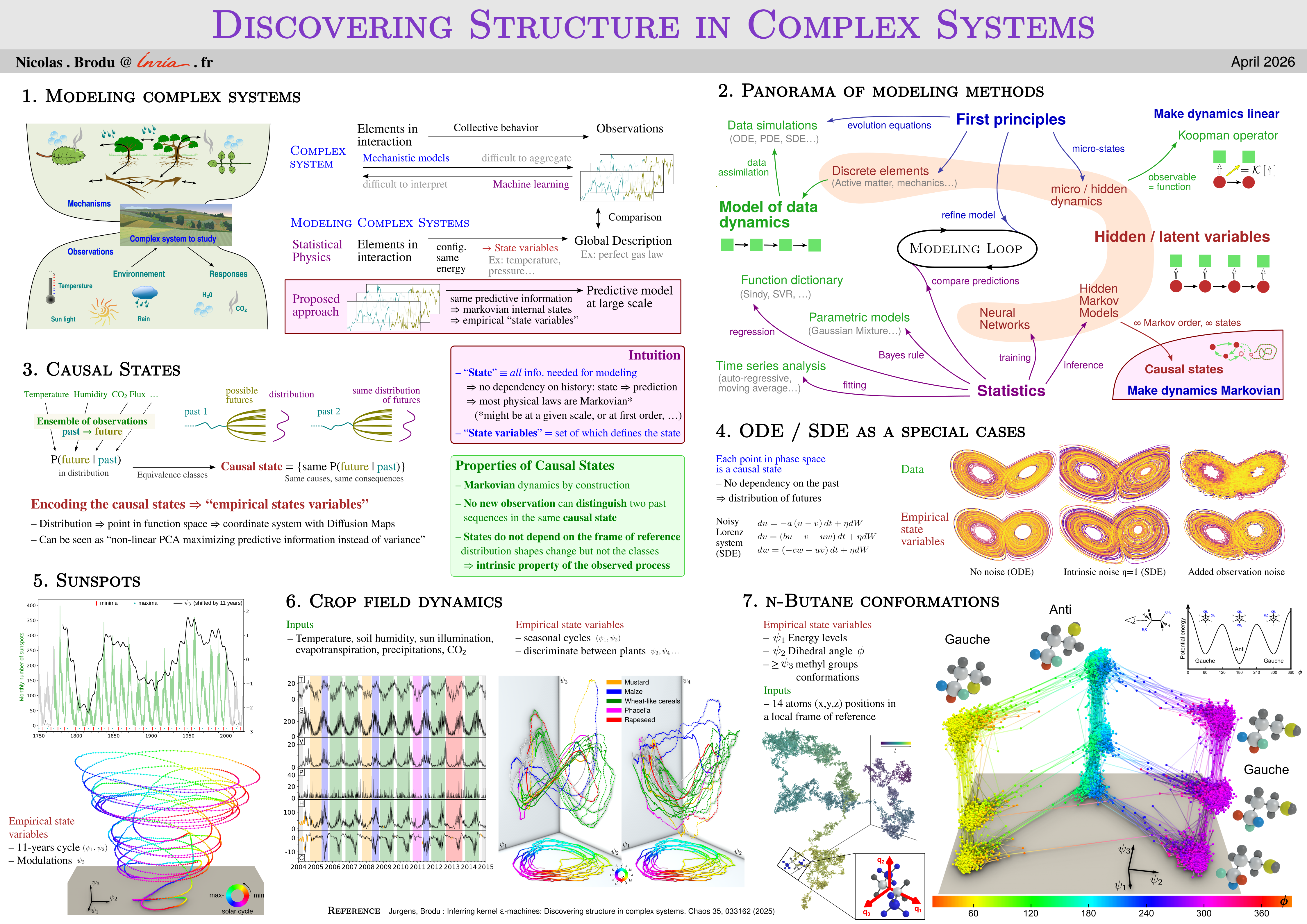
The method consists in identifying causal states: states of a process which always lead to the same kind of behaviors. The model then describes the dynamic of these states, an “equation of motion” in the causal state space. This equation describes how, starting from initial knowledge from current observations, the known information is diffused with time. As you can see in the 3D image on the right, the method also identifies the geometric structure on which causal states evolve. This corresponds to an attractor in the case of chaotic dynamical systems. As part of this process, the method identifies the main parameters (here, 3 axes X, Y, Z) that best describe the evolution of the causal states.

This framework allows in theory to quantify some important properties of a natural process. Indeed, the continuous causal states are by definition invariant by change of coordinates and they are an intrinsic property of the process which is studied. For example, it could be very useful to quantify characteristic scales, such as the mean time by which the initial information has diffused to the point that the prediction accuracy is reduced by half. Or measures of complexity, such as the difficulty to produce predictions from various measurement points. Perhaps more importantly, by varying the analysis scale, this method has the potential to identify hidden patterns in the data, the structures that bear information.

This kind of approach and variants have long been studied by many groups in non-linear physics and complexity sciences. In particular, the group of James P. Crutchfield, co-author of the first paper below and inventor of the theoretical causal states framework since the 1980's. Strong links also exist with out of equilibrium thermodynamics. What matters most for many systems of interest (the atmosphere, cells, ant colonies, etc), is the persistence of structures and their interactions through time. A model such as what is proposed here has the potential to identify and quantify the information contained at different scales. It also describes how that information is transformed.

The model proposed here does not have the ambition to solve all these issues… it is just another step – following the path shown by many groups in complexity, chaos and non-linear sciences – towards a better understanding and modeling of natural processes.

Example: analyzing solar activity

The Sun activity can be measured by counting the number of sunspots that appear each month. Periods of about 11 years are observed. The prediction of these cycles (or half-cycles…) is notoriously difficult. In order to test the algorithm and its ability to detect large-scale patterns, we are going to apply it to the long-term dynamic of the Sun. The algorithm is parameterized with the characteristic scale of 11 years: it will analyze the relation between 132 monthly measurements and the next 132 observations. Data ares collected from the SILSO resource of the Royal Observatory of Belgium. See also this paper and the matching code for a detailed analysis.

3D representation of causal states, infered from solar cycle data. The image is dynamic and you can navigate through the structure. Years of solar maxima are noted in blue and minima in black.

The method proposes a projection of causal states on a reduced set of most relevant parameters. Clearly, the first two, X and Y, encode together the 11-year period as well as the phase along the cycle. Which is expected, given this is the main macroscopic feature of this process.

Trajectories seem to all fit on a conical structure. But what is the meaning of the Z parameter, coding for the height along the cone? This parameter is identified as important by the algorithm, which puts it in third position, but I could not figure out its signification. I thus asked experts from SILSO: this parameter captures the low-frequency modulation of the amplitudes known as the Gleissberg cycle. And, indeed, dates on the lower or higher ends of the cone match these of the low-frequency modulation. So, the algorithm has also captured a pattern on a scale that far exceeds its immediate temporal horizon of 132 months! This demonstrate its ability to encode the dynamics of the process, not just the immediate statistical dependencies.

Articles and source code

Continous causal states were introduced in: Discovering Causal Structure with Reproducing-Kernel Hilbert Space ε-Machines by Nicolas Brodu and James P. Crutchfield (also available at this DOI and on ArXiv.org).

Applications were presented in: Inferring Kernel ε-Machines: Discovering Structure in Complex Systems by Alexandra M. Jurgens and Nicolas Brodu (also available at this DOI and on ArXiv.org).

The code I wrote, together with data for reproducing the figures in the second article, is available here. The previous version matching the first paper is also provided.

This is a Python package. Running the provided examples should be reasonably straightforward, with only classic dependencies (numpy, etc), but visualization helpers and figure plotters depend on external tools (plotly, pyvista). MIT License: free to use for what you want, so long as you credit the original code, but software support is not provided so you are on your own.