This is a fine comparison over the course of three months (December 2010 to February 2011) of the study site. The effect of a flood is clearly visible at the base of the cliff, showing our method has a great potential for measuring the impact of individual events. The vegetation was of course removed before the comparison as it would otherwise interfere with the measures. It is added back as post-processing.

The mountain river site laser data in 2009 and 2011, without the vegetation, has evolved much more than in the course of three months. Some parts have greatly changed (up to 7m, see below…) and others did not. In some regions the 2009 data is missing due to bad visibility. The goal is to compare both scenes in relevant directions, directly on the 3D data, to detect both large changes and small ones, to be robust to data artifacts, and to do all that in a statistically sane way.

The main difficulty is to find the relevant direction for comparing the scenes at each point, especially in the presence of measurement noise and artifacts like missing data. Intuitively the best direction is the one which is perpendicular (=normal) to the surface, which changes for each point in the data set. See on the right how the vertical component shifts from fully vertical on the river bank to fully horizontal on parts of the cliff. A tricky part not as easily seen is that the surface normal depends on the scale at which we look at the data. For example, rockfall debris are very rough when we look at them at a scale less than 1m. Let’s assume we wish to track the general change of the cliff instead of the movement of individual peebles. It is best in that case to define a direction which is perpendicular on average at a large scale, over 10m. Inversely we want to preserve details in other regions at a scale less than 10m. The algorithm thus proposes to automatically adapt the scale for defining the surface normal. It selects the scale for which the surface appears to be flattest on average, within a range given by the user (which may also be a single scale if so desired).

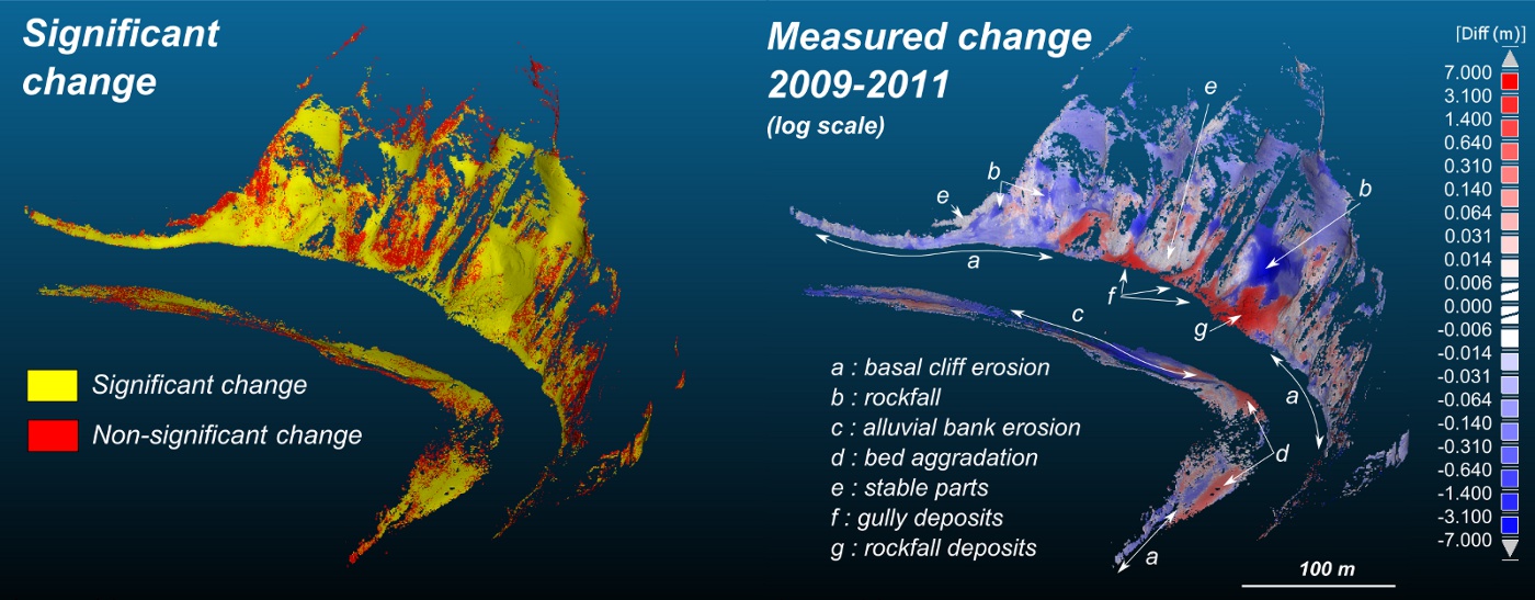
The algorithm can not only detect changes, but also give an indication as to how reliable that detection is. On the left we can see in yellow the regions where the algorithm has found interesting changes, and in red where we cannot tell if there is a change or not. On the right the interesting changes are annotated in red (more matter, like debris accumulating) and in blue (less matter, like erosion). In some regions there are very large changes (up to 7m) in two years. The algorithm precision is below the centimeter (down to about 6mm in ideal conditions). Below that precision the algorithm cannot tell whether a change occured or not. See how this corresponds to the most stable parts of the cliff.