
This new algorithm quantifies the difference between statistic properties on each side of each pixel. It realizes a kind of filter, able to detect characteristic scales in the spatial domains (e.g. in pixels) and on data values (e.g. in gray levels). The algorithm is not limited to scalar values, such as the brightness of an image. It can work directly on vector data, or many other objects for which a "reproducing kernel" is defined. It is also not limited to 2D images. Here are a few application examples, showing the versatility of the algorithm. More details explaining how this works are given below, together with the article.
Focus on either small or large variations


The algorithm allows the user to specify a characteristic data scale at which changes are sought. For example, at a scale of one gray level (second picture), the algorithm detects jpeg artifacts in the sky and around the coat. The large brightness changes are, on the other hand, completely ignored, which could be useful for example for a guided filtering of jpeg artifacts without touching large contrast variations. These are found in the third image, by specifying a data scale corresponding to the maximal black/white contrast. This last result is closer to what a classical edge detection algorithm would find, based on large gray level gradients. This ability to filter either small or large variations makes the algorithm very versatile, hence adapted to a wide range of potential applications.
Borders surrounding repeating patterns
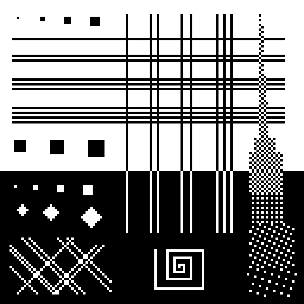
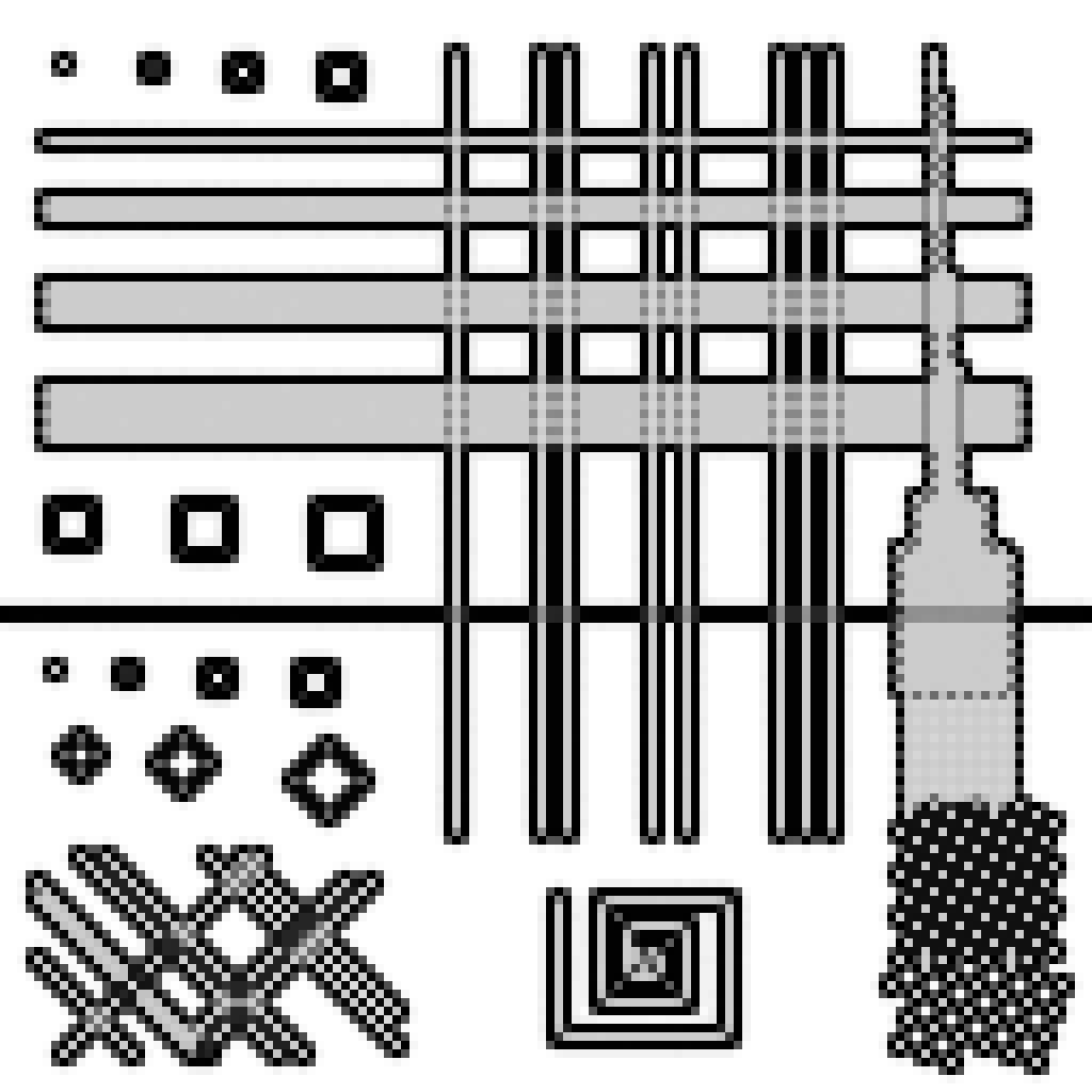
The algorithm allows the user to specify a characteristic spatial scale, at which patterns are recognized and treated as a unique texture. Here, using a scale of one pixel, a border is detected around, but not within, the horizontal lines separated by one pixel. Similarly for the chessboards on the right, where the difference is clearly visible between these using a repeating 1-pixel pattern (they are surrounded by a unique border), and these using a pattern on a larger scale (each point is then treated separately). This technique also works along diagonals, see in the lower-left corner where a unique border is defined around lines separated by one pixel but not these wider apart.
Inferring characteristic scales
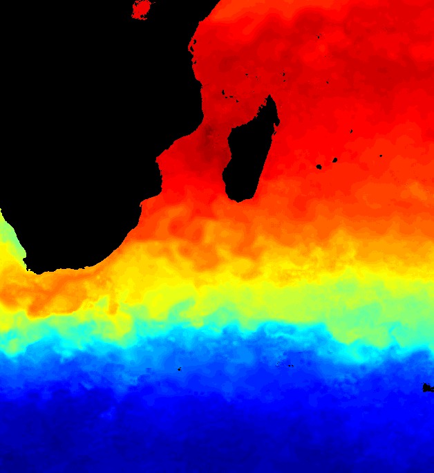
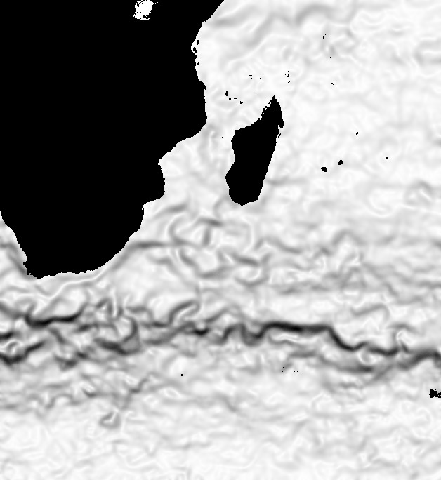
When both the spatial and the data scales are varied, we can scan which scales extract the most information in the zones detected by the algorithm. Thus, not only zones can be detected where "something happens", where information is concentrated, but we can also find what are the relevant scales for the analysis of these zones. In the above picture, these zones match oceanic currents, with a characteristic width of 75 km (at the center of the image) and for typical variations of 1°C.
Detecting borders using color information
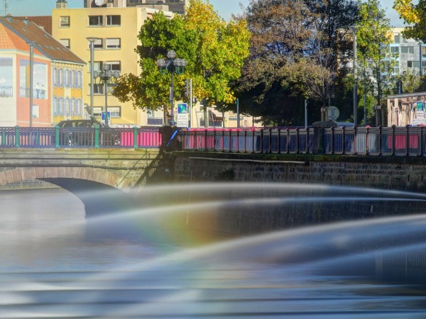
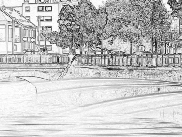
Thanks to the use of a reproducing kernel, the algorithm works directly on vectors, including color spaces. Color information is thus incorporated in the edge detection. Other vector spaces can be considered, such as multispectral or radar data, and even non-vector objects (e.g. strings). This image is an extract from a larger picture taken by Thomas Bresson, under Creative Commons - Attribution.
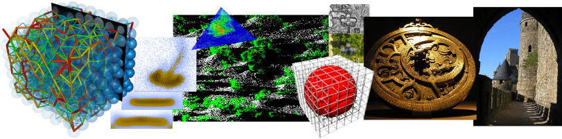
How it works
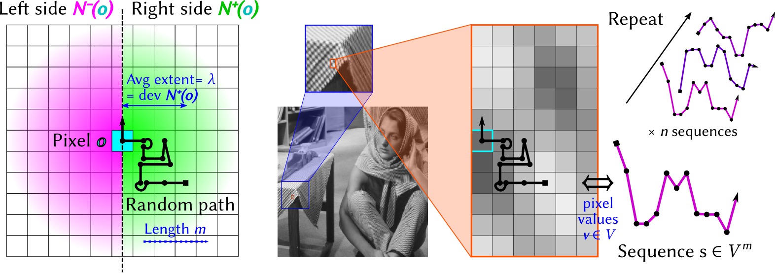
The idea is to compare statistical properties of each side of a pixel, then repeat the operation in each desired direction (e.g. horizontal, vertical, diagonals). A random path is first generated (left), with a length m and average spatial extent λ pixels. This spatial scale is also the standard deviation of the probability distribution that a pixel is included in a random path (density shown in green and pink). Pixel values v∈V along the path are then taken as a sequence in Vm.
A texture is then modeled as a probability distribution in Vm. Intuitively,
this distribution describes how pixel values evolve in the region considered. An empirical estimator of this distribution can be built from n sequences generated in Vm. The trick is to use a representation of these distributions in a reproducing kernel Hilbert space, in which the empirical estimator can be expressed very simply. Another advantage is that the norm between two points in this space quantifies directly the distance between two probability distributions, hence, in the current case, between twe textures on each side of a pixel. The size of the reproducing kernel defines the scale at which data are compared.
Article and code
A preprint version of the article is available here as well as on ArXiv.org, together with the presentation given as a keynote session at the conference Recent Advances in Electronics & Computer Engineering, January 2015.
The source code is maintained as a sub-project in Inria's gforge. I intend to provide a self-contained version when the article is published. In any case, this software is free, according to the LGPL v2.1 or more recent