Description
You'll find here an independent C++ class that can incrementally measure a system's statistical complexity. The theory behind this code has a long history, owing to research done 30 years and more ago. You can find more details in this article by Shalizi et al, or in that one, by the same author, under the section "Grassberger-Crutchfield-Young Statistical Complexity". The theory is also known as causal states, have strong roots in ε-machines, and more.
The goal of this code is to extend the method to make it incremental, so new observations are taken into account as soon as they come: the clusters are updated, and the complexity estimates are re-evaluated efficiently. Similarly, there is the possibility to remove obsolete points in the case the system is non-stationary and the old observations have become inconsistent with the new ones.
This code is autonomous (no external dependency), generic (applicable to any user type), simple to use (see below), and consists in a single header file you can directly include in your project. The algorithm is described in this article and also with more details in Section 5.1 of my dissertation. I provide the code here in the hope that it will be useful, feel free to re-use it if you wish!
Examples
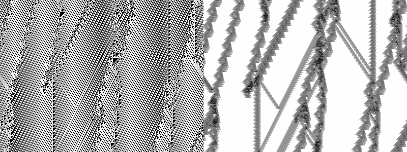
This first example shows the elementary 1-dimensional cellular automaton
(CA) for the rule 146, with random initial conditions, in a cyclic world. The left part of the image is the raw CA field, the right part shows the algorithm in action. The detected patterns are hard to follow in the CA field, but clearly visible in the complexity field. The result is comparable to the plots in this article computed with Cimula. The initial transient phase was removed and all observations were then collected before computing the complexities, using the command ./CA_Complexity -k200 -n -p6 -f6 -r146 -w400 -t300 -s11
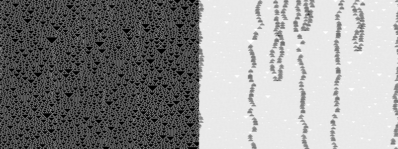
This is rule 54 in action. The image includes the random initial conditions and the observations are added row by row, incrementally: The algorithm quickly "learns" the background pattern, which is blanked out as "uncomplex". ./CA_Complexity -r54 -w400 -t300
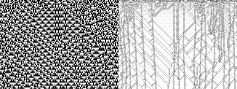
This is the famous rule 110. Transient initial conditions were skipped, and the size of the light-cones is set to make the interactions more visible. ./CA_Complexity -k500 -n -p6 -f5 -r110 -w400 -t300 -s6
The code
You can download here the latest version (1.0) containing the following files and a Makefile. You'll find in the archive:
- CausalStateAnalyzer.h: The main class. Specialize it with some past and future light cone types. Then feed it observations in the form of past/future light cone pairs. You'll get the complexity estimates incrementally updated on demand. See the quick API guide below.
- CA_Complexity.cpp: A usage example, using cellular automata. This is what produced the pictures on this page. A graphical mode is available, ./CA_Complexity -h prints an help message.
For information, the analyzer now contains a version of the incomplete gamma function optimized for its own needs. The new version was implemented from scratch, independently from any previously existing code. This avoids the need to link to an external file, like the statistical test classes from the CSSR project that were used in the first versions. The new version of the Chi-square test is both self-contained and much faster.
You can also get here the source code for the experiment described in Section 5.1 of my dissertation.
Quick API Guide
- Define your light cone types: what represent the past and future of your system. For example, integer IDs.
Then create the analyzer object:
CausalStateAnalyzer<int,int> analyzer; - Monitor your system pasts and futures and provide observed (past, future) pairs.
analyzer.addObservation(past, future); - Commit the observations when you think you have enough of them. This may be done after each pair if you wish, or once you have collected all the observations, or whenever you like.
analyzer.commitObservations(); - At the point, the complexities are ready:
The local complexities are returned as vectors with one entry for each observation pair you provided, in that order:
vector<float>& complexities = analyzer.getComplexities();
The global complexity is the amount of information in bits that would be necessary to encode all the causal states:
float globalComplexity = analyzer.getGlobalComplexity();
You may now loop to step 2 to continue providing observations, etc.
Just remember to commit the observations before reading the new complexities.
Optional:
- You can remove previous observations, which is especially helpful for (slowly) non-stationary systems where the complexity evolves over time.
analyzer.removeObservation(too_old_past, too_old_future); - You could also call the "getScaledComplexities" function to have the values in [0..1], scaled using the observed min/max. This is useful for making grayscale images for example.
vector<float>& complexities = analyzer.getScaledComplexities();
History
v1.0: No change. Renamed 0.8 to 1.0 as the code is now stable, and also symbolically for the release of my PhD dissertation and a published article.
v0.8: CA_example fixed. Slight performance increase.
v0.7: Corrected bug in distribution counts. Added features to the CA example.
v0.6: Optional: The class may now be serialized, which is especially useful for saving/restarting computations.
v0.5: Added more tests to correctly handle data removal.
v0.4: Squashed flat an horrible bug, changed to 2-step incremental API, introduced assembly optimizations, and more performances.
v0.3: Improved performance, removed dependence to CSSR test routines.
v0.2: Corrected bugs and improved performance.
v0.1: Initial public release.